Recently, I had to analyze the power profile of a microcontroller at a specific point in time. This article will cover the required steps to perform such measurements with Rigol DS1054Z/1104Z oscilloscope.
Contents:
Python interface
You can connect to the oscilloscope via USB or LAN/LXI. Since it’s only USB2.0, you might think that LAN would be much faster, however this is not the case - download speed over LAN is painfully slow.
In order to interact with the scope from python first we need to install pyvisa-py and pyusb modules via pip. Now we can send SCPI commands that are described in DS1000Z Programming Guide.
This is where things get ugly. Simple queries worked fine, but as soon as I tried to read the waveform I encountered either a timeout or the following error:
1 | usbtmc.py:115: UserWarning: Unexpected MsgID format. Consider updating the device's firmware. |
At the moment of writing the article I was using python 3.11 with pyvisa-py 0.6.2. Firmware was already up to date and increasing the timeout didn’t help at all. It seems like every time a try any python wrapper around libusb it simply doesn’t work..
After half an hour of debugging I found that setting chunk_size to 32 produces stable(-ish) results on both of my machines. If that doesn’t help, you might want to try setting RECV_CHUNK to 32 and max_padding to 0 in pyvisa_py/protocols/usbtmc.py
Collecting waveforms
Be default :WAV:DATA? command will return the on-screen memory, which is limited to 1200 points. Since we need slightly more than that, we’ll have to perform a ‘deep-memory’ read. We can read only 250k points each time, so the memory has to be read out in chunks. After some trial and error I found out that higher values like 500k work as well, although stability degrades. By ‘stability’ I mean the amount of retries required to read each chunk successfully - even 250k read might take 1-2 attempts to complete successfully.
The following script assumes that we trigger on CH2 and capture CH1 waveform. For each trace we’re arming the scope, waiting for the acquisition to complete, performing deep-memory read and dumping the results into csv file. Things like memory depth and trigger settings should be configured on the scope manually.
1 | import time |
Aligning traces
Since we’re triggering on a different channel and our event of interest occurs some time after the trigger, our traces most likely will have some misalignment due to various reasons like clock jitter, which we’ll need to learn how to deal with.
Let’s say we have two signals a and b offset by phase:
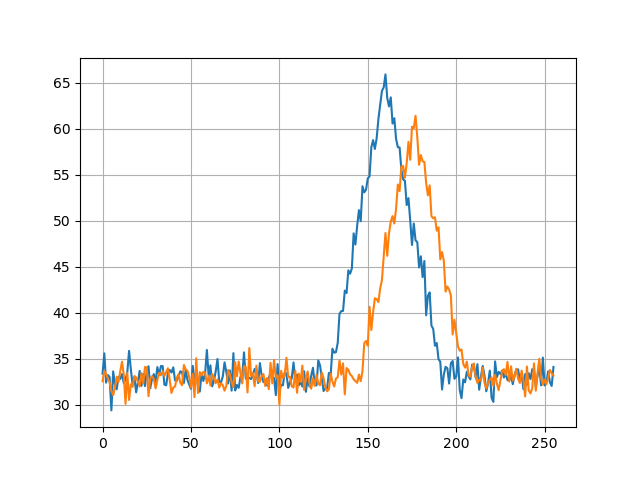
We can ‘align’ them by using cross-correlation. Applying some filtering prior to that is also a good idea, but we’ll skip this step for now. Cross-correlation doesn’t play well with signals that have some DC bias and can produce false peaks, so we remove that first. Next we find the largest peak - this is the point where our signals align.
1 | import numpy as np |

Cross-correlation produces a sequence of length 2n - 1 symmetrical around a single point with ‘zero’ being in the middle of the x-axis. Our phase shift is the x-coordinate of the maximum relative to ‘zero’. Knowing the offset, all we have to do is shift one of the signals. Obviously we loose some data after performing the shift - you can throw these points away from both traces or fill them with some fixed value instead (in this case - median).
1 | # align traces |

Processing data
Now we can process the captured traces. Of course we can load everything into memory, but in case we might need gigabytes worth of traces (good luck capturing those with this scope), we’re going to read the capture file line-by-line, align each trace with the reference trace and apply a simple moving average.
1 | import matplotlib.pyplot as plt |
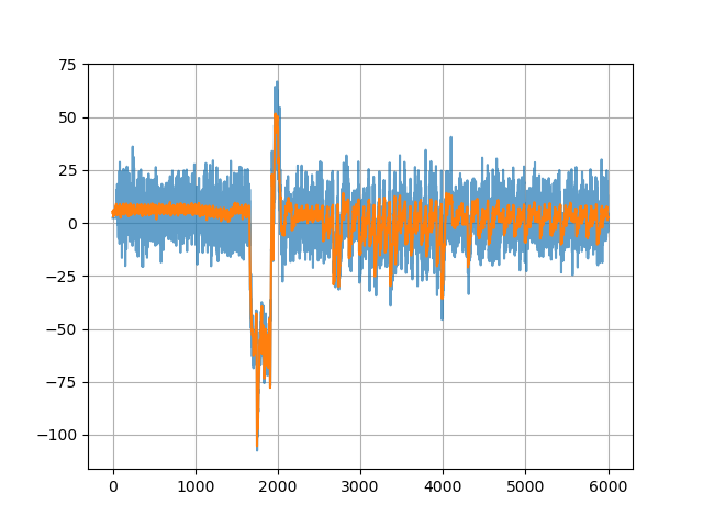
Conclusion
Even though DS1054Z is definitely not the best tool for this job, it can still get the job done, especially with a bit of patience. Below is the example of one of the sets of traces that I captured. As usual, code is on github.